I’ve been looking recently at decompositions of matrices, specifically the eigendecomposition, and the singular value decomposition (SVD). Check out my last article to see more! Today we’re specifically going to look at an example of using the eigendecomposition to remove radio frequency interference from an astronomical observation!

The eigendecomposition of a symmetric, non-negative definite square matrix says that it can be decomposed into a set of eigenvectors , and a diagonal matrix of eigenvalues :

Let’s see the power of this decomposition. What are we going to use it for? Well, in radio astronomy, we have a big problem with radio frequency interference. This is interference from a terrestrial source: a satellite, a mobile phone tower, even a microwave! This is often much more powerful than the celestial sources we are trying to observe. Currently we don’t have good mitigation algorithms for this interference, however a new type of antenna may change that: the Phased Array Feed (PAF).

The PAF’s major advantage is its many antennas. In contrast to a normal telescope that has one antenna, the PAF replaces it with a checkerboard of 188 antennas. Furthermore, the celestial source that we are observing will only appear in some of the antennas, while the interference will be present in all of the antennas. This means that we want to subtract away the common signal between all of the antennas, the interference, in order to uncover the weaker celestial signal.

Let’s take an example. I’ve simulated an astronomical signal that we’re going to bury under a huge layer of noise! This is a simulated pulsar, a type of astronomical object that gives off a signal at regular intervals. The x-axis is time, and the y-axis is the flux – think about this as how powerful the signal is.

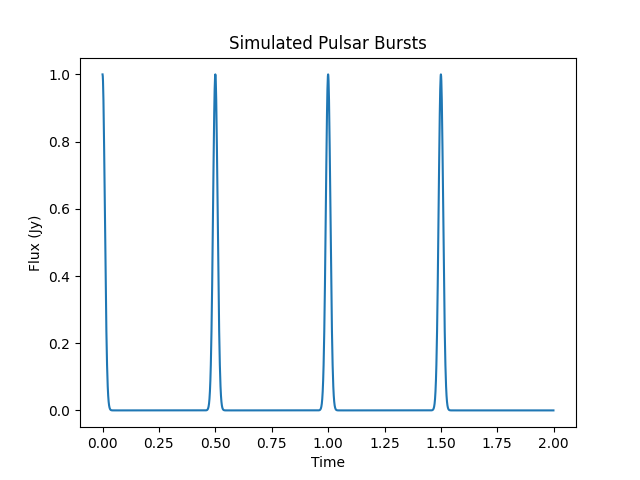
We’re also going to simulate some RFI, and this is going to be much stronger than the astronomical signal. The pulsar bursts are on the order of 1 Jansky, while the RFI is on the order of 20 Janskys!

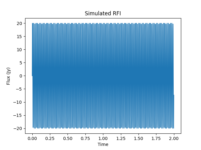
The next image shows the final signal hitting our antenna, with the signal, the RFI, and some uncorrelated noise – you can hardly see the astronomical signal!

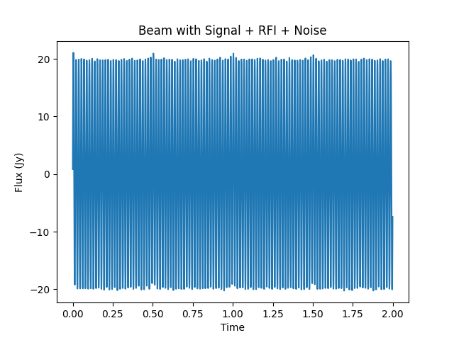
As we said above, this technique can only be used in an array of antennas. What we’re going to do is create an array of three antennas. The first antenna will get the signal that we see above, with the celestial signal, the RFI, and noise. The other two antennas will only get the RFI & uncorrelated noise. Then we’re going to use the eigendecomposition of the covariance matrix to remove the common RFI signal between the different antennas.

Setting the first eigenvalue to zero and reconstructing the time series with the new correlation matrix yields the beam below – we can see those pulsar bursts clear as day!

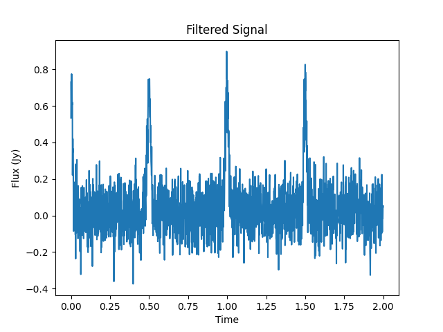
As a further check, let’s compare our filtered signal with the original signal without the RFI – just the signal + noise. The filtered signal is on top, with the original signal underneath. As we can see, they are almost identical!

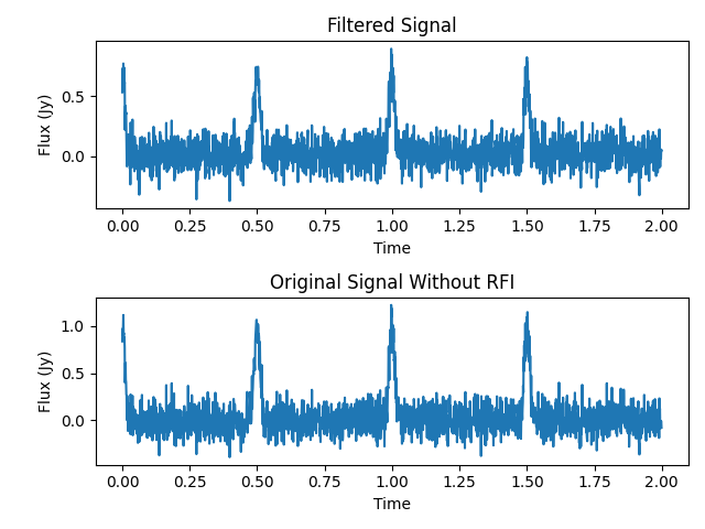
This is a very simplified example, but it does outline the immense power that linear algebra has in untangling RFI from astronomical signals!

Watch out for more articles showing how this can be used in more complex situations!

Full code for this article:

import numpy as np
import matplotlib.pyplot as plt
from scipy.linalg import sqrtm

# Simulation parameters
fs = 1000             # Sampling rate (Hz)
duration = 2          # Duration in seconds
t = np.linspace(0, duration, int(fs * duration), endpoint=False)

# Pulsar parameters
pulsar_period = 0.5   # Seconds between pulses
pulse_width = 0.01    # Width of each pulse
pulse_amplitude = 1.0

# RFI parameters (same in all beams)
rfi_freq = 60         
rfi_amplitude = 20.0   # Strong RFI

# Noise parameters
noise_level = 0.125

# Number of beams
num_beams = 3

# Generate the pulsar signal (Gaussian pulse train)
pulsar_signal = np.zeros_like(t)
pulse_times = np.arange(0, duration, pulsar_period)
for pt in pulse_times:
    pulsar_signal += pulse_amplitude * np.exp(-0.5 * ((t - pt) / pulse_width)**2)

# RFI: Same in all beams
rfi = rfi_amplitude * np.sin(2 * np.pi * rfi_freq * t)

no_rfi_real_beam = None

# Create the 3 beams
beams = []
for i in range(num_beams):
    # Add pulsar signal only to beam 0 (as only that beam sees the pulsar)
    signal = pulsar_signal if i == 0 else 0
    noise = np.random.normal(0, noise_level, size=len(t))
    beam = signal + rfi + noise
    
    beams.append(beam)

    if i ==0:
        no_rfi_real_beam = signal + noise

X = np.vstack(beams).T

# 1. Remove mean
X_mean = np.mean(X, axis=0, keepdims=True)
X_c = X - X_mean

# 2. Compute covariance matrix and its eigendecomposition
C = np.cov(X_c, rowvar=False)
eigvals, eigvecs = np.linalg.eigh(C)

# 3. Remove the first eigenvector (set its eigenvalue to 0)
eigvals_filtered = eigvals.copy()
eigvals_filtered[-1] = 0  # largest eigenvalue (last one after eigh)
C_filtered = eigvecs @ np.diag(eigvals_filtered) @ eigvecs.T

# 4. Whiten original data - remove covariances
C_sqrt_inv = np.linalg.inv(sqrtm(C))
X_white = X_c @ C_sqrt_inv

# 5. Re-correlate with modified covariance
C_filtered_sqrt = sqrtm(C_filtered)
X_filtered = X_white @ C_filtered_sqrt

# 6. Add back the original mean
X_filtered += X_mean

plt.plot(t, pulsar_signal)
plt.xlabel("Time")
plt.ylabel("Flux (Jy)")
plt.title("Simulated Pulsar Bursts")
plt.savefig("images/pulsar_bursts.png")

plt.plot(t, rfi)
plt.xlabel("Time")
plt.ylabel("Flux (Jy)")
plt.title("Simulated RFI")
plt.savefig("images/simulated_rfi.png")

plt.plot(t, X[:,0])
plt.xlabel("Time")
plt.ylabel("Flux (Jy)")
plt.title("Beam with Signal + RFI + Noise")
plt.savefig("images/beam_w_signal_rfi_noise.png")

plt.plot(t, X_filtered[:, 0])
plt.xlabel("Time")
plt.ylabel("Flux (Jy)")
plt.title("Filtered Signal")
plt.savefig("images/filtered_signal.png")

fig, axes = plt.subplots(2, 1)

ax = axes[0]
ax.plot(t,X_filtered[:,0])
ax.set_xlabel("Time")
ax.set_ylabel("Flux (Jy)")
ax.set_title("Filtered Signal")

ax = axes[1]
ax.plot(t, no_rfi_real_beam)
ax.set_xlabel("Time")
ax.set_ylabel("Flux (Jy)")
ax.set_title("Original Signal Without RFI")

plt.tight_layout()
plt.savefig("images/filtered_vs_original_beam.png")