In my PhD research, I’m seeing that the frequency domain is extremely useful for bringing insight to chaotic time domain signals.

The frequency domain is the realm of electrical signals and Fourier Analysis. While I took a course on Partial Differential Equations, it was by far the lowest mark of my mathematics courses. For years I didn’t need it, and I was content to leave that as an area on my mental treasure map that simply said “There be dragons”. Now, my PhD work means that it’s time to slay the dragons.

The Dragon’s Den

The datasets that I’m working with now are mostly voltage data from radio telescopes. They’re mostly multi-dimensional, complex (in both the mathematical and everyday sense), and rooted in the world of frequencies.

So, let’s see how and why thinking in the frequency domain is useful.

The major insight is that mathematical functions, or time series, can be broken down to be the sum of an infinite number of sine / cosine waves, being the Fourier Series of the function or time series. This means that saying I have a sine wave at 1 GHz is equivalent to presenting an entire time series. Stating only the frequencies involved brings structure to otherwise extremely chaotic datasets.

For example, here is the time domain representation of a signal I generated:

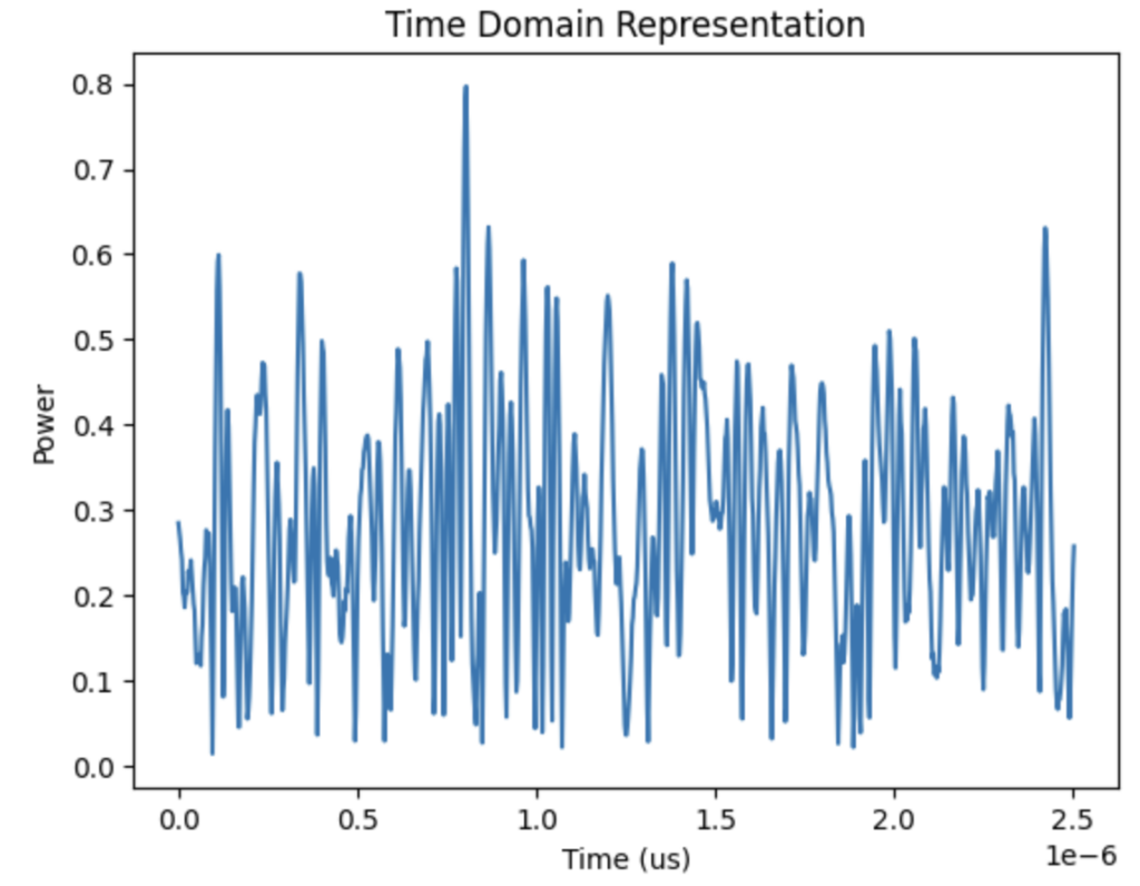
It doesn’t look like much, right? If you needed to take any insights from this, it would be pretty hard. However, if we look at this instead in the frequency spectrum:

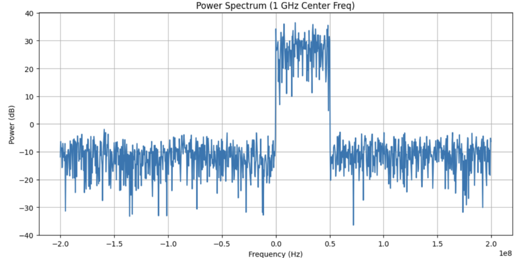
We can now see that this time series was generated by a signal with a bandwidth of 50 MHz. This means that the difference between the top frequency and the bottom frequency in the signal is 50 MHz. We can also see that the signal begins at 1 GHz. All other frequencies are just noise.

It has taken me a while to get used to this idea, and thinking in the frequency domain still does not come naturally to me. Let’s take a look at a couple of the misconceptions that I have needed to clear up in my learning journey:

Misconception 1: Sampling needs to be done at twice the frequency of the highest signal frequency that exists in your sample.
Correction 1: Sampling needs to be done at twice the bandwidth of the signal.

This misconception caused me to crash my computer trying to simulate a signal, and generally made life much harder than it should have been. Correcting this misconception taught me why it was bandwidth that was important, and not necessarily frequency.

Nyquist sampling is an important result in Digital Signal Processing (DSP) which is important to understand the connection between signals, and the sampled digital representation of that signal. Essentially it says that if you sample too infrequently, you cannot faithfully reconstruct the signal you’re trying to analyze.

This is best seen visually, so I’ve stolen an image below that shows the connection between the actual signals on the left hand side, sampled at different rates.

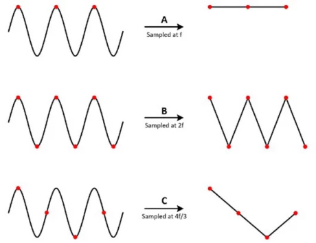
Nyquist sampling is usually stated as saying that you should sample at least twice as frequently as the highest frequency in your signal. This would lead to some pretty tricky logistical issues, however. If you wanted to simulate a 1 GHz signal, you’d need to create at least 2 billion samples per second for that signal! This is a great way to make your computer give you the BSOD.

This statement of the theorem is only true assuming that you’re analyzing a baseband signal. That is, it includes all frequencies from 0 Hz to 1 GHz. The actual statement concerns sampling at twice the bandwidth of the signal. For example, if you’re analyzing signals between 0.9 GHz and 1.1 GHz, a bandwidth of 200 MHz, then you need to sample at 2 x 200 = 400 MHz. This is still fast, but is far smaller than the 2 billion samples we would have previously created for 1 second of data.

Misconception 2: Negative frequencies are non-physical
Correction 2: Negative frequencies have physical meaning, especially when analyzing non-baseband data.

I didn’t really know how to think about negative frequencies, which caused me a lot of confusion when I got spikes in the negative portion of the power spectrum. Clearing up what these actually mean has meant that I can actually understand the spectra I’m producing.

When you take an FFT of a signal, you’ll get a series of frequencies that are centered at zero and contain both positive and negative frequencies. At baseband, i.e. 0 Hz -> some frequency, if you have a real signal then you can safely ignore the negative frequencies as they will be simply the complex conjugate of the positive frequencies.

However, if you’re using a frequency band that is not centered around zero, then your negative frequencies correspond to the frequencies below the center frequency. For example, in the previous example the -100 MHz channel will correspond to 1 GHz – 100 Mhz = 1 GHz – 0.1 Ghz = 0.9 GHz. This means that even with a real-valued signal, you can’t ignore the negative frequencies from the FFT.

Conclusion

I will continue to make mistakes in my signal processing journey, that’s unavoidable. Cataloguing them will be useful to someone who is on a similar learning path to me, as well as reinforces my own learning. So stay tuned for more articles!